Uncategorized – Page 2 – To be decided

Trump’s tweets (and the Women’s March comparison)

Posted on January 23, 2017January 25, 2017 by dtoher

So, I’ve been working on sentiment analysis again. What could be more topical than analysing the tweets from the period after Trump was elected to before he was sworn in.

I downloaded Trump’s tweets from twitter in R (from the handle @realDonaldTrump)

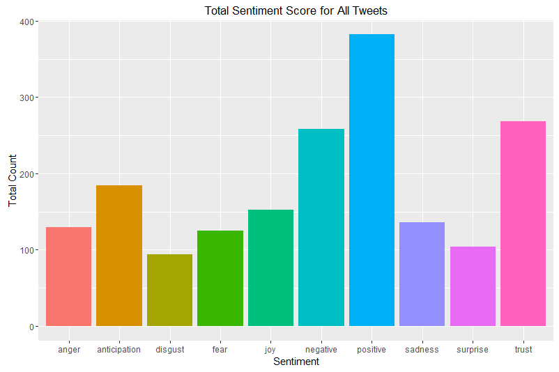
Using the syuzhet package in R it is very simple to perform sentiment analysis; with some simple manipulation afterwards, we can see the profile of the different “Sentiment Score”. A step-by-step guide is here.

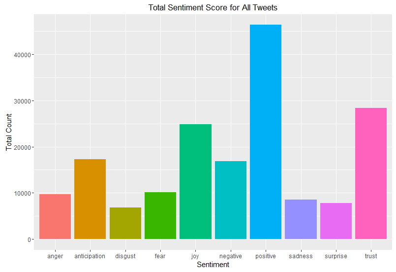
First look at the profile across all of the tweets:

trumps tweets sentiment counts

But, things with Trump are not quite that simple. It has been previously speculated that Trump’s tweets from Android devices are not written by the same person as Trump’s tweets from other sources. The general conclusion is that the tweets from Android are written by Trump himself, but tweets from other devices are written by staffers. The time of posting the tweets can be investigated to see if there are patterns:

time of Trumps tweets as President Elect

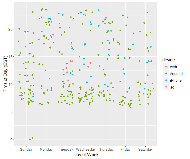
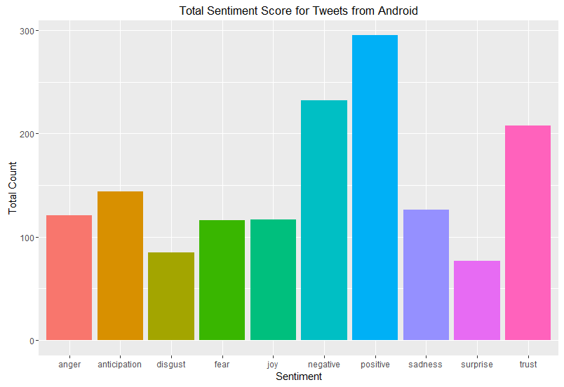
It becomes very obvious that whoever is tweeting from the iPhone is primarily active during office hours – with a few evening [18] tweets that were either thank you tweets or mentioning events that evening or the following morning. So, let’s look at those tweets written on an Android:

Number of tweets sent via an Android device with each particular sentiment

In the following sequence of wordclouds, the word in the middle corresponds to the sentiment in the graph above.

So what words were said in tweets that the sentiment analysis deemed to be angry?

wordcloud of angry Trump tweets as President Elect

Compare this to the joyful tweets:

wordcloud of joyful Trump tweets as President Elect

and the tweets expressing “trust”

wordcloud of trusting Trump tweets as President Elect

This process is continued for the other sentiments…

Who might be interested in this type of analysis? It doesn’t just apply to political figures; companies may be interested in the sentiments being expressed about their brands / services and in particular may be interested about the effects that changes have on what is being said online. Whether you are aware about it or not, this type of analysis is happening every day and is providing insight into how people think about a wide variety of terms.

There are limitations, of course. These include the problem of sarcasm and emojis. Automatic sentiment analysis struggles to capture sarcasm. Furthermore, emojis can be converted into text, but the additional meanings behind the emojis (think aubergine) are lost in this process!

Who knows what the future will bring as Donald J Trump has control over both the @POTUS and @realDonaldTrump accounts!

As a quick aside; here’s the sentiment captured between 21:57:57 and 22:40:31 UTC [about 5pm EST and 2pm PST] on Saturday January 21st under the hashtag #WomensMarch. This consisted of approximately 65 thousand tweets in total. I could have collected more data, but twitter has a limit of 5000 tweets in a single download, so it’s quite a faff to collect more. Furthermore, I didn’t think that more tweets from earlier in the day to substantially change the pattern.

The names of the “sentiments” are fixed, sometimes not exactly to my preferred choice; tweets with a high “trust” sentiment are often quite hopeful for example… but that is a whole different problem (and is someone else’s problem to worry about!)

womensmarchsentiment

Definitely a more striking ratio of positive to negative tweets.

And the most commonly used words:

Finally, for those interested in this tweet:

It came from an Android phone on a Sunday (but not very early in the morning / late at night); so those speculating that it was not the man himself tweeting don’t have the obvious indication of it coming from an iPhone!

teaching, Uncategorized

Student Projects: Spatial Statistics

Posted on January 20, 2017 by dtoher

At this time of the year, I once again start to think about how to create interesting, but feasible, projects for final year students. Many times I find students have their own particular set of interests and I will try to work through a process with them to develop project ideas that will maintain their interest for an academic year.

Recently, I have been primarily focusing on projects with a spatial element, for a number of reasons.

Goes beyond what they are taught in an particular module on their degree programme
Lots of public/government data available have a spatial element
Encourages students to use R rather than SPSS/Minitab (the other statistics packages that we teach our students)
Looks good on a CV as it is unusual to see analysis and modelling of spatial data at an undergraduate level.

I mainly recommend a single textbook to students; Applied Spatial Data Analysis with R by Bivand R.S., Pebesma E. and Gómez-Rubio V. This is a great book for those learning spatial statistics.

As we mainly use Generalised Additive Models when analysing the data, the framework that I use for explaining the concepts tend to be:

(Multiple) Linear Regression: response variable continuous, explanatory variable(s) continuous

$E[y|x]=\beta_0+\beta_{1}x_{1}+\cdots+\beta_{p}x_{p}$

General Linear Models: response variable continuous, explanatory variable(s) may be categorical or continuous
Additive Models: response variable continuous, model uses functions of explanatory variables

$E[y|x]=\beta_0 + f_{1}(x_{1})+\cdots+f_{p}(x_{p})$

Generalised Linear Models: response variable not necessarily continuous (could be binomial or poisson), explanatory variable(s) may be categorical or continuous

$g\left(E[y|x]\right)=\beta_0+\beta_{1}x_{1}+\cdots+\beta_{p}x_{p}$

Generalised Additive Models: response variable not necessarily continuous (similar to Generalised Linear Models), model (may) use functions of (some of) the explanatory variables.

$g\left(E[y|x]\right)=\beta_0 + f_{1}(x_{1})+\cdots+f_{p}(x_{p})$

This talk gives a very quick overview of GLM / GAM.

This year, I have students looking at the US Primary election results on a county-by-county level (principally examining the within-party rather than the between-party distribution of votes) and also looking at cancer rates around Europe. Previous projects have looked at more economic data with a spatial element.. but perhaps the future will involve more environmental applications.

Uncategorized

Another morning after the night before

Posted on November 9, 2016November 9, 2016 by dtoher

This time around, I didn’t wait for the election to be called. On the morning of June 24, I stayed up until the numbers of votes to be declared was less than the margin at the time. This morning, I watched the results on a county-by-county level for states like Virginia – which did veer to Clinton at the end, I could see that Clinton’s Democratic “firewall” wasn’t as solid as people were predicting. Pennsylvania was the same on a county-by-county level; even prior to full reporting, it was obvious that Trump was more popular than the polls had anticipated.

So, once again, the polling agencies have to question themselves. While many states were within the usual margin of error of polls, that the bigger errors were typically in the same direction (towards Trump) once again reveals that there are some structural issues about the performance of the opinion polls and how the polling companies capture difficult to reach voters. An even trickier issue is understanding those who lie to pollsters about their voting intentions [or, to be more generous, change their mind at the last moment] for reasons of social acceptability.

At this stage, with 31 electoral college votes still available, but with only 3 states left to declare, Trump has exceeded the required 270 electoral college votes to win [even without Washington state’s faithless elector]; but with 99% reporting, according to AP, the current state of the popular vote is:

99% reporting	Votes
Donald Trump Republican Party	47% 59,521,401
Hillary Clinton Democratic Party	48% 59,755,284
Gary Johnson Libertarian Party	3% 4,050,927
Jill Stein Green Party	1% 1,210,290
Other candidates	0.7% 798,952

Spoiler Alert?

Were any states sufficiently close as to be influenced by potential “lower order” candidates. Well, yes, quite a few, but most were votes for Gary Johnson, the Libertarian candidate – which are perhaps more likely to break towards Trump (or, more likely, not voted).

What happens if we consider Jill Stein’s voters. Suppose that she hadn’t been running, and, instead, her voters split 50/50 for Clinton [leftish] and Johnson [challenger / alternative party]

Michigan’s 16 electoral college votes [as of the current reported state of play] would be firmly in Clinton’s column, but no other states would have swung.

If, instead, the split had been 75/25 for Clinton [leftish] and Johnson [challenger / alternative party], then still only Michigan would have been in play for Clinton.

So, the splitting of the left wing vote may have cost Clinton Michigan [subject to the final votes being counted], it cannot be blamed on her losing the Electoral College.

Notes: data obtained via the AP feed (as google reports it) and via http://edition.cnn.com/election/results/president

The CNN website is particularly useful as it gives the county-by-county breakdown across (almost) all states, rather than requiring you to go to individual states webpages.

ps: I have a student who is looking at the relationship between socio-demographic variables and the primary voting patterns in a selection of US states on a county level (or town where appropriate). It will be interesting to see if anything crops up by applying similar analysis to the general election results to see if there were obvious trends [or if it is just a spatial thing] that had been overlooked during the campaign period. But that is definitely work for another day, as she has until the end of the second semester to complete her work!

Uncategorized

Clearing: Just what have I got myself into?

Posted on August 15, 2016 by dtoher

Back from my holidays, into the process of UCAS clearing. It is the first time I’ve experienced it, as I’m now a programme leader, which means that I now get some input into the relative rankings of different potential students.

Chatting with one of my colleagues at lunch today, we discussed the different systems as experienced by us. In Belgium, some courses have an entrance examination, but otherwise, on successful completion of secondary level you are qualified to enter a degree course. This slightly fills me with worry, as there must be some fierce logistical issues with having “no limits” to your potential student numbers, especially for some courses that require access to labs.

In Ireland, the system administered by the Central Applications Office [CAO] gives universities the ability to set minimum requirements in specific subjects and the total number of students that they want to recruit for a particular course. Once that process is complete, the universities essentially have no further input (there are some minor exceptions). Instead the magic of the Irish predilection for preference based systems comes into its own. Just considering the direct entry into degree level, Irish students get to rank their top 10 degree programmes. For the setting of the tariff is completely out of the hands of the universities – it is a complete supply / demand situation that governs the equivalent of the tariff attached to the courses. Provisional offers are only made for those on non-traditional entry routes, otherwise everything comes down to the students meeting the minimum requirements, the entrance examinations [for Medicine] and then allocating the number of spaces (let’s call that X) available in a manner like this:

Look at all applicants who gave your course a rank.
See who passes the minimum requirements.
Offer a place to the X best students. The lowest of them sets the “points” total.
Some students may decline their offer (for any number of reasons), even if students accept an offer, they you may receive an offer from higher up your original preference list, but not lower down your preferences…
Thus there can be many rounds of offers…

The important thing is that it is based on your results; not your personal statement, nor your personal reference, or any subjective input from people like me…

Uncategorized

More or Less

Posted on April 22, 2016 by dtoher

Today my first interview on BBC Radio 4 aired – as part of the Friday afternoon programme “More or Less”: available here

I became involved in this when a producer contacted the Royal Statistical Society who fielded it out to the Statistical Ambassadors looking for a volunteer.

What started out as a very simple listener question:”What’s my chance of being called to do jury service” from a Scottish resident threw up many different quirks of the Scottish system. In order to simplify the problem, I first decided to look at the probability of receiving a citation (the equivalent of a summons); because this part of this could be treated as an essentially random process.

The Scottish Courts service helpfully provided data on the number of citations issued and also the number of jury trials in Scotland, leading to the first quirk of the Scottish system: they have 15 rather than 12 member juries. From this we could work out the probability of being cited from the Scottish electoral register [which contains some people who are ineligible for service].

I used a poisson distribution to model the probability of receiving 0 (zero) citations in a year. For ease, I assumed that this rate was approximately constant over the range of years under investigation. This may, in reality, be a bit of a stretch for the 53 years of typical eligibility, the listener in question had only 9 more years before he could opt out for age reasons. I also assumed that the chances of receiving a citation is independent year-on-year (although eligibility is definitely not independent). I also assumed that the number of trials in a catchment area was approximately proportional to the number of people on the electoral register – again, this simplification had to be made as that was all of the available data – anything deeper would have been beyond the scope of a general audience radio programme.

Last year, only 13% of those who were cited actually served on a jury in Scotland..

Because you are exempted from jury service for a period after being balloted for service (and for even longer if you actually serve on a jury), looking at the number of times a person can serve on a jury is far more complex.

As for the experience of recording the programme. All of my interactions were with a producer (who was lovely) – many emails, several phone calls and then a trip for me into BBC Bristol to record my thoughts on a decent ISDN line. The recording took about 25 minutes in total, partially because some new questions popped up during the recording, meaning that I ran some calculations on the spot! These were condensed into about a minute on the radio. Because of the format of the show, and the fact that I was prerecorded, it wasn’t nearly as stressful as I’m sure other media experiences can be [I wasn’t there to argue or provide balance against another person].

Listening back to myself was a strange experience – I definitely moderated my voice to ensure that my accent is less pronounced and also I spoke much more deliberately than usual. Perhaps this was because I was conscious that More or Less goes out to quite an international audience (it is also broadcast on the World Service).

Uncategorized

Final Count of Seats: who won what?

Posted on March 3, 2016 by dtoher

So Longford-Westmeath results are in, so we can now look at the geographic breakdown of the final votes and seats in the Irish General Election:

Beginning with the most important: who won seats where?

In the next two plots, the size of the pie-chart are proportional to the number of seats being contested (so Dún Laoighaire was adjusted to only have 3 out of 4 seats contested as the Ceann Comhairle is returned automatically). Renua won no seats (so the colour orange is slightly redundant in these legends!)

SeatsWon-Dublin

Dublin: Labour won no seats south of the Liffey; but the Greens won two. Social Democrats won one seat in Dublin; Fine Gael won at least one seat in every Dublin constituency (and two in Dún Laoighaire and Dublin Bay South). Fianna Fáil improved their lot over 2011 when they won a single seat in Dublin – now they have 6 seats in Dublin. PBP-AAA won 5 seats in total in Dublin while Sinn Féin won 7. Independents also won 7 seats in Dublin.

SeatsWon-RoIreland

Interesting constituencies include Tipperary: 3 out of 5 seats were won by Independent candidates and Roscommon-Galway where 2 out of 3 seats were won by Independents.

Fine Gael managed to return at least one TD in all of the other constituencies (barring the two with two with a majority of independent seats), with two returned in Wexford, Kilkenny-Carlow, Limerick County, Clare, Galway-West, Mayo, Wicklow, Meath-East and Louth.

Fianna Fáil returned at least one TD in all non-Dublin constituencies, with two in Cork South-Central, Cork North-West, Kilkenny-Carlow, Kildare South, Kildare North, Cavan-Monaghan, Sligo-Leitrim and Mayo.

Sinn Féin won two seats in Louth and one in: Donegal, Sligo-Leitrim, Cavan-Monaghan, Meath West, Offaly, Laois, Wicklow, Kilkenny-Carlow, Limerick City, Kerry, Cork North-Central, Cork South Central, Cork East and Waterford.

All the counts in one place

politics, Uncategorized

Transfer Politics

Posted on March 1, 2016March 2, 2016 by dtoher

One of the unusual features of the Irish electoral system is that of transferable voting. Since the constituencies (other than in by-elections or in Presidential elections) have more than one seat to be filled, the bigger parties often run more than one candidate.

They often try to spread the candidates out geographically throughout the constituency, in order to try to capture geographic transfers as well as party transfers.

Using an example, from a 3-seat constituencies: Cork North West, I will explain how the transfer system works. The calculation for the quota (the point at which a candidate is elected) is as follows:

$\frac{NVotes}{NSeats+1}+1=\frac{NVotes}{4}+1$

where NVotes is the number of valid votes, and NSeats is the number of seats being contested. Thus in the case of a three seat constituency, a candidate has to accumulate one vote more than 25% of the number of valid votes to be automatically elected [note that this doesn’t apply at the final count, as some votes are not transferred and so the effective number of votes is reduced].

CorkNorthWest

Count 1: All number 1 preferences are counted for each candidate.

At the end of Count 1, in the case of Cork North West, no candidate was elected, so they decided to eliminate candidates. In this case the three candidates (O’Donnell, Griffin and O’Sullivan) with the fewest 1st preferences were eliminated together.

Why aren’t they eliminated one at a time? Well, consider the case of the four lowest polling candidates:

Green Party: C. Manning 1354
Independent: J. O’Sullivan 478
Independent: S. Griffin grey 439
Communist Party: M. O’Donnell 185

The sum of 2-4 on this list is 1102. So therefore, if they were to be eliminated one at a time, and all the transfers went to the next highest in the queue – so all O’Donnell’s 185 1st preference votes were transferred (by expressing number 2 preference) to Griffin (to result in a value of 624 votes for Griffin) and then O’Sullivan is eliminated (still having only 478 votes, having received no direct transfers from Griffin) and all O’Sullivan’s votes also go to Griffin, Griffin would still only have 1102 votes, which is less than Manning’s 1354.

Therefore, after Count 1, all of the ballot papers that had 1st preferences for O’Sullivan, Griffin or O’Donnell are then examined and the 2nd preferences are looked at. The votes are then literally transferred into the candidates’ that received the number 2 rank pile of ballot papers.

At the end of Count 2, still no one has reached the quota, so Manning (the remaining candidate with the fewest votes) is eliminated. Any of Manning’s votes that attempt to make their next preference for one of the already eliminated candidates have their next available preference considered. Note that, since a Supreme Court judgement, if a voter forgets to include a preference – so gives ranks 1-3, forgets 4, restarts at 5, then all preferences after 3 are deemed invalid and the vote becomes non-transferable.

This process continues until Count 8, when a candidate is elected (if more than one is elected on the same count, the one with the greater surplus is considered first; if the excess is so small as to not to make a difference to potential order of elimination/election, they may choose to go straight to the next elimination). Counters look at the last pile of votes added into Creed’s pile of votes – the transfers from Collins, another candidate from the same political party. They look at all the next preferences in this pile and then split the number of excess votes in proportion to the next available preference (after Creed). In this case, the majority of these went to O’Shea. The votes they choose to distributed the excess from are randomly sampled [so as they do not consider lower order preferences, this could, potentially effect who are elected] – but it did not matter in this case, as Count 9 was the last count.

In this count, A. Moynihan exceeded the quota and was deemed elected.

M. Moynihan was then elected without them checking A. Moynihan’s excess as M. Moynihan was sufficiently far in excess of the only other remaining candidate (O’Shea) that it would not have made a difference, even in the unlikely event that all of A. Moynihan’s votes went to O’Shea (although of the same party, the two Moynihans are not related). Thus M. Moynihan was elected without making the quota, because, by Count 9 there were 3,650 untransferred votes, making it impossible for the final person elected to exceed the quota.

politics, Uncategorized

On Voting: different systems

Posted on February 25, 2016March 2, 2016 by dtoher

It’s Irish election time; causing me to think about the differences between the UK and Irish election systems for general elections.
UK’s First Past the Post system means that most voters are really voting for a party rather than a candidate. There are safe seats where candidates without any attachment to the constituency can be parachuted in and win. For all the attachment to constituency based politics, I’ve heard little from candidates despite living in a relatively unsafe seat.

Ireland’s Proportional Representation via Single Transferable Vote in multi -seat (3, 4 or 5 seats) constituencies means that there are no fundamentally safe seats. In constituencies that a party is popular in often more than one candidate from the same party is on the ballot paper. This lack of safe seats leads to a lot more clientism and localism in Irish TDs (MPs).

Ideally those elected should contribute to the good of the entire country, not just their constituency, but the Irish system doesn’t necessarily encourage that type of behaviour among voters.

2011	1st Preferences	% of 1st Preferences	Number of Seats	% of Seats
Fine Gael	801,628	36.1	76	45.8
Fianna Fáil	387,358	17.4	20	12.0
Sinn Féin	220,661	9.9	14	8.4
Labour	431,796	19.4	37	22.3
Others	378,916	17.1	19	11.4

Transferring of votes is very important when considering electoral success in Ireland. Fine Gael (and to a lesser extent Labour) did well – gaining a greater percentage of the seats in the Dáil than would be expected on a purely proportional split of votes. Indeed, they encouraged transfers of votes between the two parties (once their own list of candidates was exhausted).

Quotas in Irish General elections are as follows:

3 seat constituencies: (25% (1/4) of the valid votes)+1 vote
4 seat constituencies: (20% (1/5th) of the valid votes)+1 vote
5 seat constituencies: (1/6th of the valid votes)+1 vote

The final seat often does not make the quota due to people not having a full ranking of candidates (so the effective quota reduces). This makes the last seat the seat most dependent on the success of a candidate at attracting votes from others. This has been a traditional problem for Sinn Féin – them failing to attract transfers in the same numbers as other parties (this happened in the last Dublin South-West by-election)

Fianna Fáil did particularly poorly in Dublin in the 2011 election – returning just a single seat:

IrishElection07-seats-Dublin — Number of Seats per party in each Dublin Constituency

Comparing that to the relative share of 1st preference votes; we can easily see what a disaster Dublin was in 2011 for Fianna Fail.

IrishElections07-1stpref-Dublin — 1st preference vote share: pie charts are proportional in size to the number of valid votes

In the rest of Ireland, this trend was echoed, but not to the same extent:

IrishElection07-seats-country — Number of seats returned in each non-Dublin constituency

Compared to vote share of 1st preferences:

IrishElections07-1stpref-country — 1st preference share by constituency

It will be interesting to see how this changes with the results over the weekend. The fragmentation of votes has been predicted by polls and media, but whether this will continue down to the vital second, third and fourth preferences will only reveal itself over the weekend.

Uncategorized

Video based learning materials

Posted on November 21, 2015 by dtoher

From recent discussions with students it has become obvious that where previously the first port of call for students trying to understand a method would have been their notes, followed by recommended textbooks, students are turning away from the written word [in statistics / mathematics at least].

Which leads me to think about what type of material is best conveyed through the medium of video rather than as static text.

For a number of years, I have been recording derivations done (generally aimed at final year mathematics undergraduate students). I try to keep these to under 10 minutes in length, but when I review average watch duration, it is under 3 minutes. Having thought about this carefully, I can’t see a way to shorten these videos without loosing important details.

These videos, considering how niche the target audience is, have proven to be surprisingly popular. Looking at when during the year the peak viewing figures are, they nicely correspond to when most students would be first introduced to the material and then again when they would be revising for examinations. An example of one such video is below:

I’ve also begun to start recording screen demonstrations of how to do different statistical analyses in Minitab and SPSS. This includes not only the basic “how to” but also how to then appropriately edit the resulting output for professional looking reports. These are pitched at second year mathematics students and also at students on MSc programmes in Biology style subjects doing Research Methods courses. For clarity, I keep these on a seperate youtube channel; an example which is feedback for a piece of 2nd year coursework is below:

https://youtu.be/rnnzkqra46I

But this leads to a problem: how do I do the same for R? Beyond the very basics of the initial set up, R is very much a command line, and hence text based language. Despite much trial and error, I’m still struggling to make good videos without spending a huge amount of time on each. The problem is that I’m essentially just commenting on code. It is rather unnatural for me to do this of any other way than by text as it would be much faster to read the text based comments than to listen to the same comments being made on a video.

I prefer to create my R scripts during my videos. I don’t like to “pre-script” the videos as my voice becomes flat rather than conveying enthusiasm. My current major issue with this is that the audio track of the videos are full of sounds of me hitting the keyboard. So I will give it one final attempt with a different keyboard, but otherwise I am stumped at how to deliver effective instructional videos for R. The other alternative is to use pre-written R scripts, but I’ve found this to be a less dynamic solution.